Designing a classifier gate for undefined regression targets
When two thirds of your targets are undefined rather than missing, imputation and sentinel values both fail. A classifier gates the regressor, and its errors are asymmetric.

Of 40.9 million training examples generated from a harvest cost simulator, 25.6 million had no cost. Not a null to impute, not a failed run to retry. The operation those rows describe cannot be performed, so the cost of performing it is undefined. Deciding what to do with that is the main architectural decision in the model, and it is made before any hyperparameter is touched.
The problem
The simulator takes a forest stand, a treatment prescription and a harvesting system, and returns a cost per green ton. For most combinations it returns nothing instead, because the combination is not physically valid: the slope is too steep for ground-based equipment, there is too little biomass to justify moving machinery in, or a safety limit is exceeded.
That is 62.5% of the generated examples.
The tempting move is to treat those rows as missing data and reach for the standard playbook: drop them, impute them, or encode the absence as a sentinel value. All three are wrong here, and for the same reason. Missing data means a value exists and you failed to observe it. These values do not exist. The distinction sounds pedantic and it determines the architecture.
Consider what each option produces.
| Approach | What the model learns |
|---|---|
| Drop the rows | Trained only on feasible cases, silently returns a plausible cost for impossible ones |
| Impute a mean | A steep-slope cluster gets an average cost, and appears in supply |
| Sentinel value like -1 | A regressor must fit a step discontinuity between -1 and $7, distorting nearby predictions |
| Sentinel value like 9999 | Same, worse, and dominates the loss |
The sentinel options fail because a regression model fits a continuous function. Asking it to output either a smooth cost surface or a fixed flag depending on a hard constraint gives it a discontinuity to smooth over, and it smooths over it, producing intermediate values that mean nothing.
What a two-stage architecture is
Split the prediction into the two questions the simulator itself asks in sequence.
Stage one is a binary classifier over all 40.9 million examples. Is this combination feasible at all?
Stage two is a regressor over the 15.3 million feasible examples only. Given that it is feasible, what does it cost?
At inference, only combinations that pass stage one reach stage two.
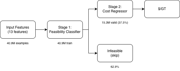
Three things fall out of this, and they matter in roughly this order.
The output space stops being discontinuous. Each model has one job with a well-formed target. The classifier predicts a label that genuinely is binary. The regressor predicts a cost over a range where a cost always exists. Neither is asked to represent "this does not apply."
The stages can be tuned against different objectives. A classifier optimised for recall and a regressor optimised for absolute error are different optimisation problems, and separating them means neither compromises for the other. This is the part that generalises furthest.
The class imbalance disappears rather than being managed. There is no reweighting, no resampling, no focal loss, because there is no longer a single model trying to fit a majority class of undefined targets.
The pattern is not specific to simulators. Anywhere the target variable has a domain over which it is not defined, and where that domain is itself predictable from the inputs, the same split applies. Predicting time-to-event when the event may never occur. Predicting price for a transaction that may not clear. In each case the gate is a real model with its own error, not a preprocessing step.
What the classifier costs
On 8,184,774 held-out examples, the production classifier reaches 99.82% accuracy, precision 0.9961, recall 0.9991, F1 0.9976.
The aggregate number is less interesting than its composition. 14,599 errors total: 11,870 false positives and 2,729 false negatives.
That ratio is a choice, and it is worth being explicit about which way it was made and whether it was made correctly.
A false negative is a feasible cluster the classifier rejects. That cluster is excluded from the supply pool, so procurement draws from slightly further away and costs slightly more. The error is invisible, conservative, and small at this scale.
A false positive is an infeasible cluster the classifier accepts. It is passed to the regressor, which returns a cost, and that cost enters a supply curve. Phantom supply appears in the answer, at a location where the operation cannot actually happen.
The model was tuned for recall, so false positives outnumber false negatives four to one. The stated reasoning is that missing feasible supply is the more damaging error. That is defensible for a screening tool where an analyst checks the shortlist afterwards. It is less obviously right for a system that returns a delivered cost to a planner, because 11,870 phantom clusters are 11,870 places where the answer is confidently describing an operation that cannot occur.
At 11,870 out of 8.18 million the practical effect is negligible, and any individual query touches a few thousand clusters at most. The point is that the aggregate accuracy figure hides which direction the model is wrong in, and the direction is the part a downstream consumer needs to know.
Model choice for stage one came down to speed rather than accuracy. Four algorithms were compared and three of them were within 0.06 percentage points of each other on accuracy. Per-prediction latency spanned an order of magnitude: 1.61 microseconds for the production model against 68.55 for a neural network. Across 165 million combinations that difference is the whole runtime budget.
Where it breaks
Errors compound across stages. A combination has to survive the classifier and then be priced correctly. Reported regression accuracy is conditional on the classifier having been right, so the end-to-end error rate is worse than either number alone. Neither model's metrics express this, and nothing in the pipeline reports a joint figure.
The gate is invisible downstream. By the time a supply curve is built, filtered combinations are simply absent. There is no signal distinguishing "the classifier rejected this" from "this cluster is not in the data," which makes a systematic classifier failure in some region hard to notice.
Stage two never learns near the boundary. Training only on feasible examples means the regressor has no exposure to marginal cases. When a false positive arrives at inference, it is extrapolating, and its output has no meaningful bound. Passing the classifier's confidence into stage two as a feature, or refusing to price low-confidence cases, would help. Neither is implemented.
The split assumes feasibility is learnable and cheap. It is here, because feasibility follows from slope and biomass thresholds the model recovers easily. If the gate were as hard to predict as the target, two models would just be two problems.
Method details at /docs/harvest-cost-method.
References
Fight, R.D., Hartsough, B.R. and Noordijk, P. (2006). Users Guide for FRCS: Fuel Reduction Cost Simulator Software. USDA Forest Service, Pacific Northwest Research Station.
Chen, T. and Guestrin, C. (2016). XGBoost: A Scalable Tree Boosting System. KDD '16, 785–794.
Ke, G. et al. (2017). LightGBM: A Highly Efficient Gradient Boosting Decision Tree. Advances in Neural Information Processing Systems, 30.