Developing hierarchical spatial indexing for Hex drill-down
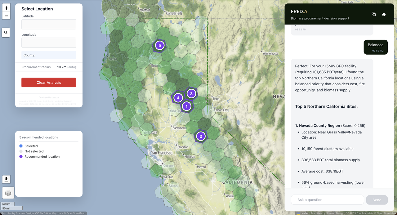
Asking "where in Northern California" means aggregating millions of spatial records with no filter to narrow them. Pre-aggregating into three hexagon resolutions turns that into three lookups under 2 ms each, and the coarse answer constrains the fine one.

Most spatial queries have a location in them. "Cost near Quincy" gives you a point, and a bounded radius around a point is cheap on any indexed table. The expensive question is the one with no point in it: "where in Northern California should this go?" That query has to consider every candidate, and there are 11.9 million of them.
The problem
A facility siting query that arrives without coordinates cannot use a spatial filter, because there is nothing to filter around. The naive implementation aggregates the full table, groups by some region, and ranks. On 11.9M rows with a spatial index that goes unused, that is seconds of work, and it happens on the first turn of a conversation, before the user has told you anything useful.
Worse, the aggregation unit is usually wrong. Grouping by county is convenient because county boundaries are in the data already. But counties in California range from 120 to 52,000 square kilometres, and a county average tells you almost nothing about where inside it to put a plant. In one benchmark query the regional average understated the best available site by 6.8%. The good hexes were there. The aggregation hid them.
What hierarchical hex indexing is
A discrete global grid system tiles the earth in cells at a fixed set of resolutions, where each cell at resolution n has a defined parent at n-1. H3 (Uber) uses hexagons, which have the property that all six neighbours are edge-adjacent and equidistant. Square grids do not: a square has four edge neighbours and four corner neighbours at a different distance, which distorts anything involving adjacency or radial growth.
Three resolutions are used here.
| Resolution | Approx. cell diameter | Role in a query |
|---|---|---|
| R4 | 22 km | Statewide overview, first pass |
| R5 | 8 km | Regional candidates |
| R6 | 3 km | Precise siting |
Each resolution has its own pre-aggregated table: mv_hex_r4, mv_hex_r5, mv_hex_r6. Every row holds one hex with its total biomass, mean harvest cost, mean burn probability, and the fraction of clusters reachable by ground-based equipment. Building them is a one-time cost paid at data load rather than per query.
A lookup then hits a table with thousands of rows instead of millions:
SELECT hex_id, parent_hex, total_biomass_bdt, mean_cost, ground_fraction
FROM   mv_hex_r4
WHERE  ST_Intersects(hex_geom, :region_geom)
ORDER  BY mean_cost
LIMIT  10;
That returns in under 2 milliseconds.
Why the live aggregation fails
It is not only slow. The deeper problem is that a single aggregation forces one choice of granularity, and the right granularity depends on the answer.
Aggregate coarsely and you get fast results that hide the variation you care about. Aggregate finely and you are back to scanning millions of rows to rank candidates that are mostly irrelevant. Neither setting is correct for the whole query, because the query has two phases: narrow the region, then find the spot.
Precomputation at multiple resolutions lets each phase use the granularity that suits it. The cost is storage and staleness. Three materialised aggregates have to be rebuilt when the underlying prediction layers change (PostgreSQL documentation), which is fine when the layers are regenerated in batch and would not be fine if they updated continuously.
Drill-down inside one conversation
The hierarchy is what makes the phases connect. Each R4 result carries a parent_hex reference, and the agent uses it to constrain the next query rather than starting over.
Turn 1  find_best_locations(region="Northern California", resolution=4)
        → 5 candidate R4 hexes, ranked

Turn 2  find_best_locations(parent_hex=<best R4>, resolution=5)
        → R5 hexes inside that one cell only

Turn 3  find_best_locations(parent_hex=<best R5>, resolution=6)
        → 3 km siting candidates
The search space collapses by roughly an order of magnitude at each step, and no step ever touches the cluster table. The user experiences it as a conversation that gets more specific, which is what they wanted anyway.
Location-free queries average 14.2 seconds end to end, the fastest of any query type in the benchmark, with the fastest completing in 4.4 seconds. They are faster than queries that name a location, because a named location triggers geocoding and then full cluster retrieval, while a location-free query can answer from aggregates alone until the user commits to a site.
Where it breaks
Hexagons do not nest exactly. This is the one thing to know before using H3 for anything quantitative. A hexagon cannot be tiled by smaller hexagons, so an R5 cell's seven children do not exactly cover its parent; they overlap the boundary slightly. Aggregates are assigned by cell centroid, which means a cluster near a boundary can be counted in a parent whose child it does not fall inside. At R4 to R6 with the cluster densities here the effect is small, but it is a real source of drift between resolutions, and it would matter if you were summing biomass across the hierarchy and expecting the totals to reconcile.
A coarse cell can be good on average and bad everywhere specific. A 22 km hex with a low mean cost may be averaging cheap valley floor against expensive slope. Drill-down recovers this, but a user who stops at R4 and reads the number as a site estimate will be wrong. The interface reports R4 results as regional summaries rather than site costs for this reason.
Rebuild cost is not trivial. Regenerating three aggregate tables from 11.9M rows takes minutes, so any change to the cost or fire layers means the hex views are briefly stale.
More on how facility siting queries work.
References
Uber Technologies. H3: A Hexagonal Hierarchical Geospatial Indexing System. Documentation.
PostGIS Project Steering Committee. ST_Intersects. PostGIS documentation.
PostgreSQL Global Development Group. Materialized Views. PostgreSQL documentation.