Retrieval over prediction surfaces, not documents
Standard RAG retrieves passages. Some questions need numbers that do not exist until you compute them. CS-RAG retrieves from three model surfaces over 11.9M spatial records, then computes before the model writes anything.

A planner asking where to put a 25 MW biomass facility near Quincy needs a number that is not written down anywhere. It has to be computed at the moment the question is asked, from three separate model outputs that have to be read at the same location simultaneously. Retrieval augmented generation in its usual form cannot answer this, because it assumes the answer already exists in a document and the only hard part is finding it.
The problem
Three models produce the inputs to a siting decision. A gradient boosted surrogate predicts harvest cost for every forest cluster in California under every treatment and harvesting system. A USDA FSim raster gives annual burn probability. A terrain zone model gives the circuity factor, the ratio between road distance and straight line distance, which converts a map distance into a haul distance.
None of the three answers the planner's question. The answer is a supply curve: sort every cluster within some radius by delivered cost, take them in order until annual demand is met, and report what the last tonne cost. That calculation needs all three layers read jointly at every cluster, and it does not exist until someone runs it.
This is a different shape of problem from the one RAG was designed for (Lewis et al., 2020). The knowledge is not text. Retrieval is not similarity search. And the retrieved material is an input to a computation rather than context for a paraphrase.
| Dimension | Standard RAG | Tool-augmented (ReAct) | CS-RAG |
|---|---|---|---|
| Knowledge source | Text corpus | Arbitrary data | ML prediction layers |
| Retrieval mechanism | Embedding similarity | Tool call | Spatial radius query |
| Post-retrieval step | None | Tool result | Domain computation |
| Output type | Text response | Text response | Decision plus rationale |
| Domain expertise | User-supplied | User-supplied | Agent-autonomous |
The distinction from ReAct is not tool calling. It is what sits behind the tools, and what happens after retrieval.
What a spatial prediction layer is
A spatial prediction layer is a function from a geographic location and a parameter set to a value, materialised in advance as a surface over a discrete spatial index rather than evaluated on demand.
Written generally:
L : S × Θ → Vwhere S is the geographic domain, Θ holds parameters like treatment and harvesting system, and V is the value domain.
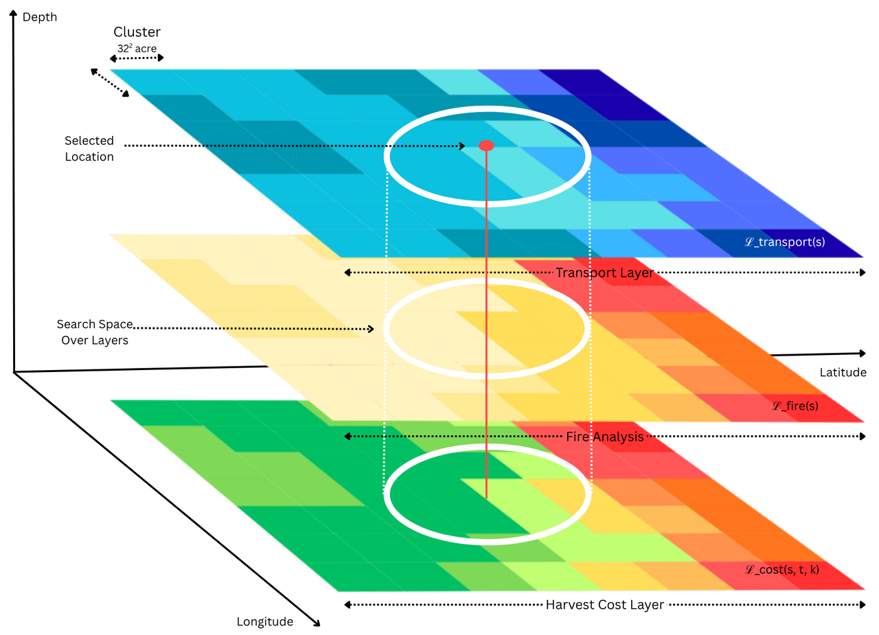
Three layers are defined.
| Layer | Value | Source | Storage |
|---|---|---|---|
| Cost | Harvest cost per cluster, by treatment and system | XGBoost surrogate over FRCS | mv_cluster_supply, 11.9M rows |
| Fire | Annual burn probability | USDA FSim raster, joined to clusters | mv_cluster_supply, same rows |
| Transport | Circuity factor by terrain zone | Five zones interpolated from 445k routes | cluster_cf_lookup, 1.53M rows |
Cost and fire share a table because they are always read together. Circuity lives separately because it is a property of the origin zone rather than of the cluster, so many clusters share one value.
All three are keyed on cluster_no and carry GIST spatial indexes, which means the joint read is one query:
SELECT s.cluster_no, s.harvest_cost, s.burn_probability, cf.circuity_factor
FROM   mv_cluster_supply s
JOIN   cluster_cf_lookup cf USING (cluster_no)
WHERE  ST_DWithin(s.geom, ST_MakePoint(:lon, :lat), :radius_deg);
Precomputation is doing the load bearing work here. The alternative is calling the underlying simulator at query time, and a single facility analysis needs tens of thousands of sequential simulator calls. A twenty year projection needs an order of magnitude more. Building the surfaces first is not a performance optimisation. It is what makes a conversational response possible at all.
Why embedding retrieval fails here
The obvious baseline is to embed the system documentation in a vector store and retrieve passages. That system was built and it answers questions about methodology perfectly well. What it cannot do is return a number, because no passage contains the delivered cost at Quincy for a 25 MW plant. The failure is structural rather than a matter of tuning: there is no chunk to retrieve, no embedding to match, and no amount of reranking produces a supply curve.
Tool augmented agents get closer (Yao et al., 2023; Schick et al., 2024). They can call a function and use the result. The gap is what the tools reach: general tool use assumes arbitrary data sources and returns the tool output more or less directly to the model. Here the tools read model prediction surfaces and then run a domain computation on what came back, and the computation is where the answer is actually produced.
Standard ranking metrics do not transfer either. Precision@k (Manning et al., 2008) measures whether the right documents were surfaced. There are no documents, so accuracy has to be measured against simulator output instead, which is a separate problem worth its own post.
The four-stage pipeline
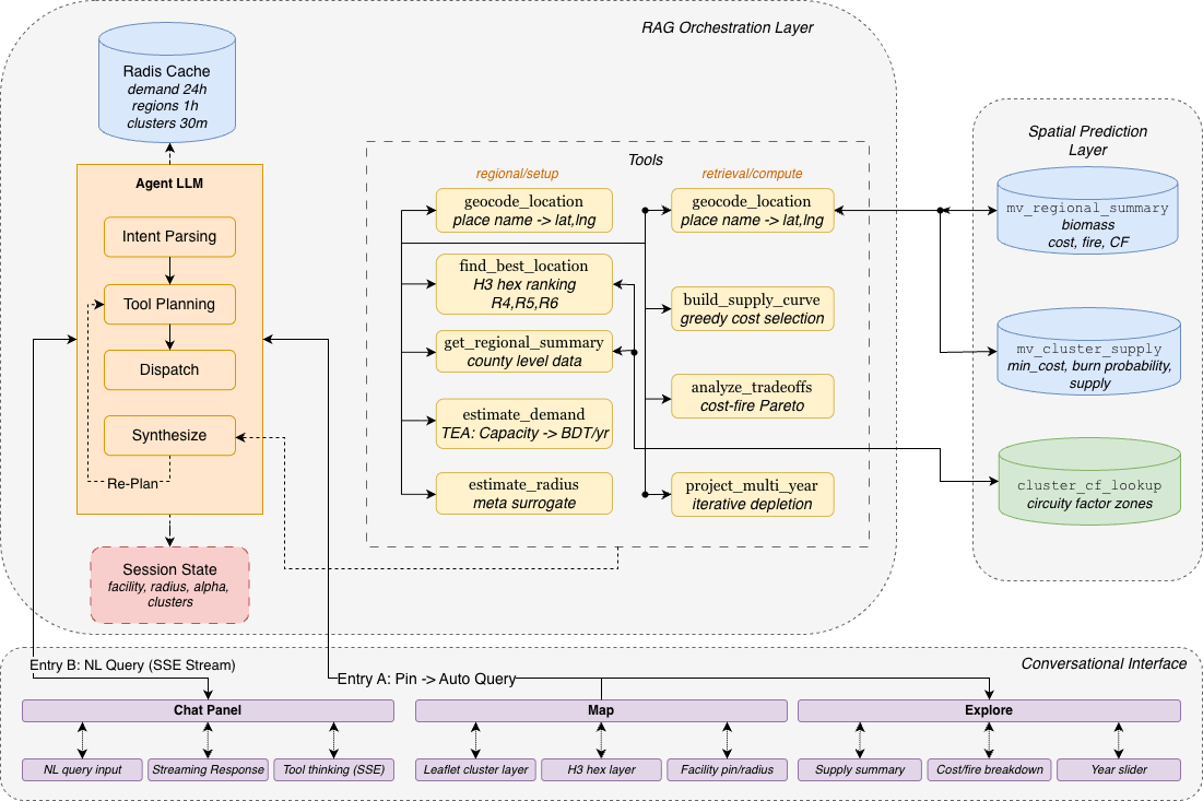
A query moves through four stages.
Intent parsing. The agent maps natural language onto a structured parameter object: location, capacity, conversion technology, fire weighting, treatment. Anything unspecified is inferred from domain defaults rather than asked about.
Spatial retrieval. Tools issue radius queries across all three layers, returning the joint set of clusters within the procurement radius.
Domain computation. Supply curve construction, Pareto sweep over the cost and fire weighting, levelised cost estimation. None of this has an analog in standard RAG.
Language synthesis. The model writes a recommendation from structured outputs, not from retrieved prose.
The delivered cost per cluster combines two of the three layers directly:
u_i = harvest_cost(s_i) + tau * haversine(s_i, facility) * circuity_factor(s_i)Under fire aware procurement the score becomes a weighted blend of that cost and the burn probability, clusters are sorted by score, and selection proceeds greedily until demand is met.
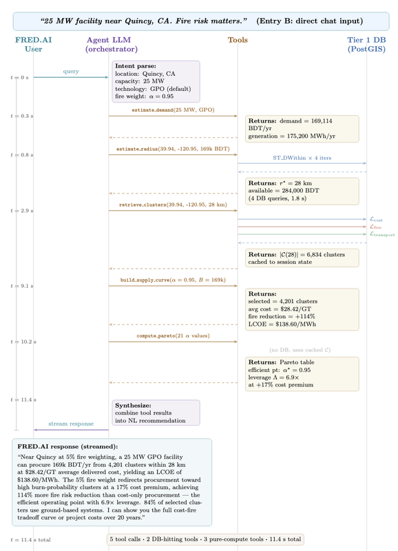
The trace above is the query "25 MW facility near Quincy, CA. Fire risk matters." Five tools run in 11.4 seconds. retrieve_clusters pulls 6,834 clusters from the joint three layer query at a 28 km radius, and everything after that computes on the cached result set. That split matters: retrieval is the expensive step, so a follow up turn that only changes a parameter skips it entirely.
Where it breaks
Transport accuracy is radius dependent, and the dependence is severe. Inside 30 km, transport cost error against full routing is 5.5%. Beyond 40 km it is 94.5%. The cause is the zone model: long hauls run on regional highways with far lower circuity than the zone average, so applying a single zone factor overestimates distance badly. Any query with a procurement radius past roughly 30 km should be read as approximate on the transport component. A distance stratified lookup would fix it and has not been built.
Two of 55 benchmark queries did not complete the tool pipeline. Both stalled because the agent asked for clarification rather than guessing, which is the preferred failure, but it is still a failure from the user's side.
Harvest costs come out 12 to 41% below the reference simulator at the same locations. That gap is not surrogate error. The reference implementation selects clusters by proximity and this one selects by cost rank across a wider area, so the two are solving slightly different problems and the cheaper answer is the correct one for the question asked. Worth knowing before comparing the two systems directly.
The methodology behind each layer is documented, and the transport approximation specifically.
References
Lewis, P. et al. (2020). Retrieval-augmented generation for knowledge-intensive NLP tasks. Advances in Neural Information Processing Systems, 33, 9459–9474.
Yao, S. et al. (2023). ReAct: Synergizing Reasoning and Acting in Language Models. ICLR.
Schick, T. et al. (2024). Toolformer: Language Models Can Teach Themselves to Use Tools. Advances in Neural Information Processing Systems, 36, 68539–68551.
Manning, C.D., Raghavan, P. and Schütze, H. (2008). Introduction to Information Retrieval. Cambridge University Press.
PostGIS Project Steering Committee. ST_DWithin. PostGIS documentation.
Fight, R.D., Hartsough, B.R. and Noordijk, P. (2006). Users Guide for FRCS: Fuel Reduction Cost Simulator Software. USDA Forest Service, Pacific Northwest Research Station.