Greedy selection with an expanding radius
Selecting the cheapest subset that meets a target, where evaluating a candidate is expensive and the pool is unbounded. The buffer is the interesting part, and greedy has a cost that arrives twenty years late.

The problem: pick the cheapest subset of candidates that meets a quantity target. Classic, easy, solved. Now add three complications. The candidate pool is unbounded, so there is no set to enumerate. Evaluating one candidate's cost is expensive. And whatever you select this year is unavailable for the next thirty.
Each of those changes the algorithm. The third one changes what "correct" means.
The problem
A facility needs a fixed tonnage of forest biomass per year. Candidates are forest clusters, each with a biomass yield and a delivered cost, where delivered cost is harvest cost plus hauling. Minimise total cost subject to meeting demand.
Written out, it is a binary integer program:
minimise    sum over i of  z_i * (harvest_i + transport_i)
subject to  sum over i of  z_i * biomass_i  >=  B
            z_i in {0, 1}
Exact solution over the full candidate set is intractable at this scale, and that framing understates the difficulty. The real obstacle is not the combinatorics. It is that computing harvest_i requires a simulator call and transport_i requires a routing call, so every candidate you consider costs milliseconds before the optimiser has even looked at it. The expensive part is populating the problem, not solving it.
That reshapes the goal. You are not looking for the optimum. You are looking for the smallest set of candidates you can afford to evaluate that still contains a good answer.
Phase one: expanding the radius
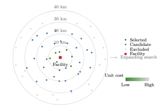
You cannot evaluate everything, so you have to bound the candidate set spatially. But bounding it requires knowing how far out you need to go, which depends on how much biomass is nearby, which you do not know yet.
Grow the boundary until the constraint is satisfied:
def gather_candidates(facility, demand, alpha=1.5, used=set()):
    r = 0
    candidates = set()
    while total_biomass(candidates) < alpha * demand:
        r += 1000  # metres
        candidates |= clusters_within(facility, r) - used
    return candidates
Two details in that loop matter more than the loop itself.
The expansion factor. The search does not stop when biomass reaches demand. It stops at 1.5 times demand. That buffer looks like slack and it is doing something specific.
Cost does not increase monotonically with distance. A cluster 12 km away on gentle terrain with good road access can be cheaper delivered than one 4 km away on a steep slope requiring cable yarding. Stopping the search the moment nominal demand is met means the selection phase never sees those cheaper distant candidates, and the greedy sort operates on an artificially truncated pool.
So the buffer is not a safety margin against running short. It is there so that the sort has something to choose from. That distinction is worth carrying to other problems: when a search bound and a selection criterion disagree about what "near" means, the bound has to be loose enough for the criterion to work.
Fixed increments, not doubling. Rings grow by 1 km at a time. Geometric growth would reach the target in fewer iterations, and it would overshoot, pulling in candidates that then have to be evaluated. When the per-candidate cost dominates, minimising iterations is the wrong objective. Minimising candidates evaluated is the right one.
Phases two and three: evaluate, then sort
Evaluation runs the cost simulator and the routing engine per candidate, computing a unit cost in dollars per tonne. This is where the time goes.
Selection is then a sort and a scan. Order by unit cost ascending, take clusters until cumulative biomass meets demand, stop.
Greedy is exactly right for this shape of problem. The constraint is a simple quantity threshold, items are effectively divisible at this granularity since one cluster is a small fraction of annual demand, and there are no interaction effects between selections within a year. Under those conditions greedy is optimal for the single-period problem, not merely a heuristic.
The phrase doing the work is within a year.
Phase four: the part that is not local
Move-in cost, the expense of physically transporting harvesting equipment to each site, is not per-cluster. It depends on the route through all selected clusters, which makes it a travelling salesman problem over the selection.
It is approximated with nearest-neighbour tour construction scaled by an equipment-specific factor. Nearest-neighbour is a weak TSP heuristic, typically 25% above optimal, and it is fine here because move-in is a small share of total cost and because the alternative is solving a TSP inside an already expensive loop.
The structural point is that this cost is computed after selection, on a set chosen without any knowledge of it. Greedy selection by unit cost has no way to prefer a spatially clustered set over a scattered one, so it will happily pick clusters spread across a wide area when a tighter group at marginally higher unit cost would have had lower total cost once move-in is counted. Nothing in the algorithm sees this.
Where greedy actually fails
Selected clusters are locked out for thirty years, the regeneration period. So year one's selection constrains year two's, and the years are not independent problems.
Greedy takes the cheapest material first. By construction, that leaves the expensive material for later.
A 25 MW facility in Butte County, run over twenty years:
| Year | Avg. distance (km) | Harvest ($/BDT) | Transport ($/BDT) | Total |
|---|---|---|---|---|
| 2025 | 5.6 | 32.68 | 9.78 | 42.50 |
| 2027 | 8.7 | 40.50 | 15.46 | 56.00 |
| 2030 | 8.6 | 37.90 | 16.48 | 54.42 |
| 2033 | 10.8 | 88.89 | 21.83 | 110.78 |
| 2036 | 12.4 | 79.57 | 27.07 | 106.70 |
| 2039 | 13.9 | 80.32 | 32.30 | 112.67 |
| 2042 | 14.6 | 117.73 | 35.33 | 153.14 |
| 2044 | 16.0 | 94.53 | 38.76 | 133.35 |
| Average | 11.6 | 65.78 | 24.83 | 90.66 |
Cost rises 3.1× over the facility's life. Year one screens at $42.50 per tonne. The twenty-year average is $90.66, more than double, and the levelised cost of electricity lands at $142.72 per MWh, likely above contract ceilings.
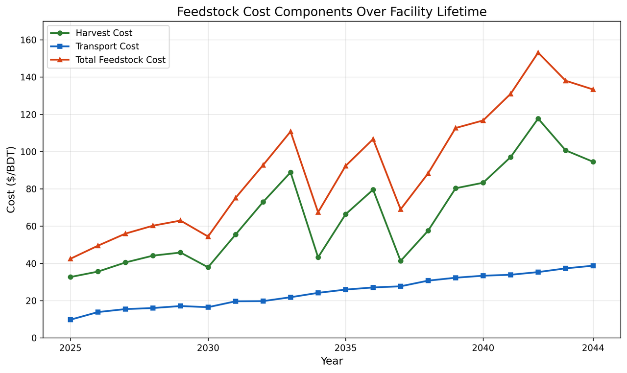
Two features of that trajectory are worth reading carefully.
Transport rises smoothly because the radius grows smoothly, from 5.6 km to 16.0 km.
Harvest cost moves in steps. The 2027 to 2030 dip is the search reaching a new band of accessible ground-based terrain. The jump from $54 to $111 between 2030 and 2033 is ground-accessible supply running out and the algorithm switching to cable and helicopter systems, which cost fundamentally more.
That step is the whole finding. It is not gradual degradation. It is a phase transition in which equipment class is viable, and no amount of extrapolating from years one through five predicts it.
The general lesson: greedy on a depleting resource is myopically optimal and globally poor, and the failure is invisible for as long as you only measure the first period. A lookahead policy that deliberately mixed expensive material into early years would flatten the trajectory and cost more up front. Whether that is preferable depends on the discount rate, which is a financing question rather than an algorithmic one.
Where this breaks
Move-in is optimised after the fact, or rather not at all. Selection cannot see the cost that depends on the selection's geometry.
Nearest-neighbour TSP is weak. Acceptable given move-in's share of total cost, and it would matter more for equipment classes with high mobilisation costs.
The expansion factor is a constant. 1.5 statewide, applied identically where terrain is uniform and where it is highly heterogeneous. It should be terrain-dependent and it is not.
No lookahead. The algorithm is aware of depletion only in that it excludes used clusters. It never trades present cost for future availability.
Thirty years is a single number. Regeneration times vary by forest type, treatment intensity and site productivity. One constant covers all of it.
The trajectory is deterministic. No fire, no mortality, no market change, no policy shift over twenty years. A twenty-year projection with no stochastic component is a scenario, not a forecast, and should be read as one.
More on multi-year projections and how delivered cost is built up.
References
Li, Y. et al. (2022). Biomass Electricity in California. Referenced in the FRREDSS 2.0 framework.
Fight, R.D., Hartsough, B.R. and Noordijk, P. (2006). Users Guide for FRCS: Fuel Reduction Cost Simulator Software. USDA Forest Service.
Short, W., Packey, D.J. and Holt, T. (1995). A Manual for the Economic Evaluation of Energy Efficiency and Renewable Energy Technologies. NREL.
OpenStreetMap contributors. Open Source Routing Machine.