Designing the record your whole system depends on
A billion 30 m pixels became 2.1 million records at 360 m. That choice was made early, propagates into every downstream model, and cannot be revisited cheaply.

Before any model is trained, something has to decide what a row is. That decision gets made early, usually while the interesting work still feels far away, and then every model, query and API downstream inherits it. Getting it wrong is not a bug you fix later. It is a schema migration across everything you have built.
The problem
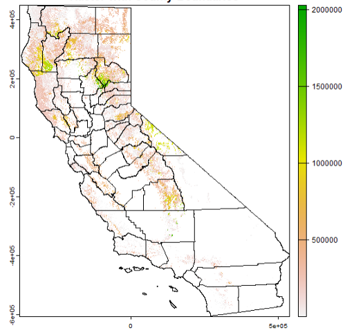
The source data is a raster. California's forest biomass inventory reports, for every 30 metre pixel across 33 million forested acres, the biomass present by component: stem wood in three diameter classes, branches, foliage. It does this separately for each of eleven possible silvicultural treatments.
That is roughly a billion pixels, and it is the wrong unit for the question being asked.
A 30 metre pixel is 0.22 acres. Nobody harvests 0.22 acres. Nobody hauls from it, sites a landing for it, or writes a contract about it. The unit the data comes in and the unit the decision happens in are different, and the gap between them is not a formatting problem. Every operational attribute that matters, road access, terrain slope, whether a machine can physically work the ground, is undefined at pixel scale because it is a property of an area large enough to work.
Storing a billion rows is also just expensive. But if that were the only issue the answer would be better hardware, and it is not the only issue.
What granularity buys and costs
The aggregation unit chosen was 360 metres, roughly 32 acres, which reduces a billion pixels to 2.1 million cluster records.
That number is a compromise between two failure modes, and it is worth being explicit about both because the reasoning transfers.
Too fine and the unit does not support the attributes it needs to carry. A landing point, the roadside location material is hauled to, is meaningless for a quarter-acre patch. Slope averaged over 0.22 acres is noise. And the record count makes the cross product unmanageable: a billion clusters times eleven treatments times ten harvesting systems is not a table anyone queries.
Too coarse and the averaging destroys the variation the decision depends on. Terrain in the Sierra Nevada changes fast. A unit spanning a valley floor and a canyon wall reports a mean slope that describes neither, and the harvesting system chosen from that mean will be wrong for both halves.
360 metres sits where a unit is large enough to have a meaningful road access point and small enough that terrain within it is roughly homogeneous. It is a judgement, not an optimisation, and the honest description is that it was chosen by domain reasoning rather than derived.
The four attributes, and why each aggregates differently
A cluster is not an average of its pixels. Four attributes are derived, and only one of them is a mean.
Biomass, by area-weighted average. Per size class, separately. Summing would double-count where pixels partially overlap the cluster boundary; averaging by area and multiplying by cluster size gives a total that reconciles.
Forest type, by plurality. Categorical data has no mean. The dominant type wins, and the minority types are discarded. This is the lossiest step and it is the one to be suspicious of: a cluster that is 51% one type and 49% another is recorded as homogeneous.
Landing point, by nearest-road query. Not an aggregation at all. It is a spatial join against the road network, producing a single coordinate per cluster. Every transport calculation in the system starts from this point, so a landing placed on the wrong side of a ridge produces a haul distance that is wrong by kilometres and there is nothing downstream that would catch it.
Terrain, from a digital elevation model. Slope and yarding distance derived from elevation over the cluster footprint. These determine which harvesting systems are feasible: ground-based below 40% slope, cable from 40 to 80%, helicopter above that. A slope error near a threshold flips a cluster between two systems whose costs differ substantially.
The general point: aggregation is per-attribute, and the correct operation depends on what the attribute means. Reaching for a groupby and taking means across the board would be wrong on three of these four.
Treatment-adjusted, not raw
The structural decision that matters most is easy to miss.
Each cluster does not carry one biomass vector. It carries eleven, one per treatment, and each describes what that treatment removes rather than what is standing there.
The same cluster under a light thin-from-below shows about 16.5 tons per acre of small-diameter stem wood. Under a clearcut it shows 34.3 tons per acre spread across all size classes. Same location, same forest, different numbers, because the prescription has already been applied.
| Raw inventory | Treatment-adjusted | |
|---|---|---|
| Rows per cluster | 1 | 11 |
| What it describes | Standing forest | Material removed |
| Prescription logic lives in | Downstream consumers | The data |
The second layout costs eleven times the storage and it removes an entire class of error. If each consumer had to apply the prescription itself, every consumer would need the silvicultural logic, and any inconsistency between them would produce numbers that disagree with no obvious cause.
It also has a consequence nobody planned. When a model was later trained to predict harvest cost, the integer treatment identifier turned out to carry 0.01% of the predictive signal, because the biomass features already encoded the treatment completely. The identifier was a label for a transformation whose output the model could see directly. That is a schema decision paying off in a place it was not designed for.
The projection, which is where this usually goes wrong
The source raster uses an equal-area continental projection, appropriate for computing areas across a large region. Coordinates are transformed to WGS 84 latitude and longitude at ingestion.
This is a two-line detail and it is the single most common way spatial pipelines fail silently. A coordinate in metres and a coordinate in degrees are both plausible-looking numbers. Join two datasets in different projections and you get results, not errors, and the results are wrong by anywhere from metres to hundreds of kilometres depending on where you are.
The rule that avoids it: transform once, at ingestion, and store in exactly one projection. Not at query time, not in the application layer, not sometimes. Every spatial join afterward is then between two things known to be in the same coordinate system, and there is no place for a mismatch to hide.
Area calculations that need equal-area properties transform back explicitly where they happen, which is a visible operation rather than an ambient assumption.
What the unit costs downstream
2.1 million clusters is not the number anything actually uses. 1.53 million have valid burn probability. Of those, 1.16 million have at least one feasible harvesting system, and 371,000 are untreatable under every treatment. The record count you design for is not the record count you query.
The untreatable clusters are not random. Their mean burn probability runs 17% higher than treatable ones, because inaccessible terrain is both hard to harvest and prone to burn. Any analysis of fire-aware procurement is conditional on a filter that systematically removes the highest-risk land, and that is a property of the unit definition as much as of the terrain.
The cross product is what you are really storing. 2.1 million clusters times eleven treatments times ten harvesting systems is the space every downstream model has to cover. Choosing a finer cluster would have multiplied all of it.
Where this breaks
Within-cluster variation is gone and there is no record of how much there was. A cluster spanning a slope break reports one slope. Nothing stores the variance, so no downstream consumer can tell a homogeneous cluster from a heterogeneous one. Retaining a dispersion measure per attribute would have cost little and was not done.
Plurality forest type discards minority composition entirely. Mixed stands are recorded as pure.
The landing point is a single coordinate with no confidence attached. Nearest road by distance is not necessarily nearest road by access. A road across a stream with no crossing is nearest and unusable.
360 metres was never validated against alternatives. No comparison of 180 m or 720 m against downstream accuracy exists. The choice is defensible and it is not measured, so the claim is that it works rather than that it is optimal.
Reversing it is impractical. Every model, every materialised view, every index and every API contract assumes this unit. Changing it means regenerating the entire prediction stack.
More on the underlying methodology and the terms used here.
References
Schatz Energy Research Center (2020). California Biomass Residue Emissions Characterization (C-BREC) Model. Cal Poly Humboldt.
Riley, K.L., Grau, D. and Scott, J.H. (2019). TreeMap 2016: A Tree-Level Model of the Forests of the Conterminous United States. USDA Forest Service.
LANDFIRE. Existing Vegetation Type. USGS and USDA Forest Service.
Jenkins, J.C. et al. (2003). National-Scale Biomass Estimators for United States Tree Species. Forest Science, 49(1), 12–35.