Estimating road distance without a routing engine
A routing call costs 50 to 200 ms and a procurement analysis needs thousands. Precomputing the detour ratio as a spatial property turns each one into an indexed lookup.
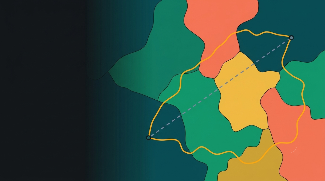
Straight-line distance between two points is free to compute. Road distance requires a routing engine, and a routing engine call takes 50 to 200 milliseconds. That is fine for one query and ruinous for a procurement analysis, which needs the distance from a candidate facility to every forest cluster around it, and then needs to do that again for the next candidate facility.
The problem
The shape of the cost is quadratic. For each candidate location, thousands of destination distances have to be routed individually. Ten candidate sites against five thousand clusters is fifty thousand routing calls, which at 100 ms each is well over an hour of wall clock for something a planner expects to be interactive.
The standard workaround is a circuity factor: a multiplier applied to straight-line distance to approximate road distance.
road distance ≈ circuity factor × straight-line distancePublished defaults sit around 1.21 nationally, and urban studies put the range between 1.20 and 1.45. Apply the multiplier, skip the routing engine, move on.
Across 435,848 measured truck routes in California's forested regions, the mean is 2.19, and the values run from 1.22 to 9.68. A national default applied to this terrain underestimates road distance by roughly half, systematically, in exactly the places where transport is the largest cost component.
Reframing the quantity
The useful move is not a better constant. It is noticing that circuity might be a property of a location rather than of a route.
If detour is a property of the origin-destination pair, there is nothing to precompute: every pair needs its own measurement, and the problem stays quadratic. If it is mostly a property of where the trip starts, then each location can be characterised once and the characterisation reused for any destination. Quadratic collapses to linear.
A pilot on 30,000 routes from 15 origins decomposed the variance by feature group. Origin features accounted for 87%. Destination features accounted for 5%.
The physical reading is straightforward once stated. Terrain around the origin determines what local road network a truck has to negotiate to reach the regional highway system. Getting out is the hard part. Once on the highway, routing to anywhere is comparatively direct, so the destination barely matters.
That result is what makes precomputation possible, and it also has consequences for how you sample, which is a separate post.
Building the estimator
Four steps.
Sample the origins. A 12 km grid over California's forested regions gave 4,127 candidate points. Removing water bodies, islands and routing failures left 3,191 valid origins. Water accounted for 387 of the 936 rejections.
Route from each one. A local OSRM instance on the October 2024 California OpenStreetMap extract, with a custom Lua truck profile: 80,000 lb gross vehicle weight, speed penalties on grades above 6%, preference for designated truck routes. Destinations were stratified across four distance bands from 0 to 150 km, which covers the range of economically viable biomass hauls. After quality filtering, 435,848 routes, averaging 137 per origin.
Interpolate to a surface. Origin-level mean circuity interpolated to a continuous 1 km raster by inverse distance weighting, power 2, 50 km search radius, both selected by cross-validation.
Cut the surface into zones. Jenks natural breaks into five classes, which minimises within-class variance and maximises between-class variance.
| Zone | Terrain | CF range | Mean CF |
|---|---|---|---|
| 1 | Flat, dense road network | under 1.5 | 1.22 |
| 2 | Valley margins, gentle slopes | 1.5 to 2.0 | 1.75 |
| 3 | Mid-elevation | 2.0 to 2.5 | 2.21 |
| 4 | Steep, sparse roads | 2.5 to 3.5 | 2.85 |
| 5 | Remote mountain | 3.5 and above | 4.84 |
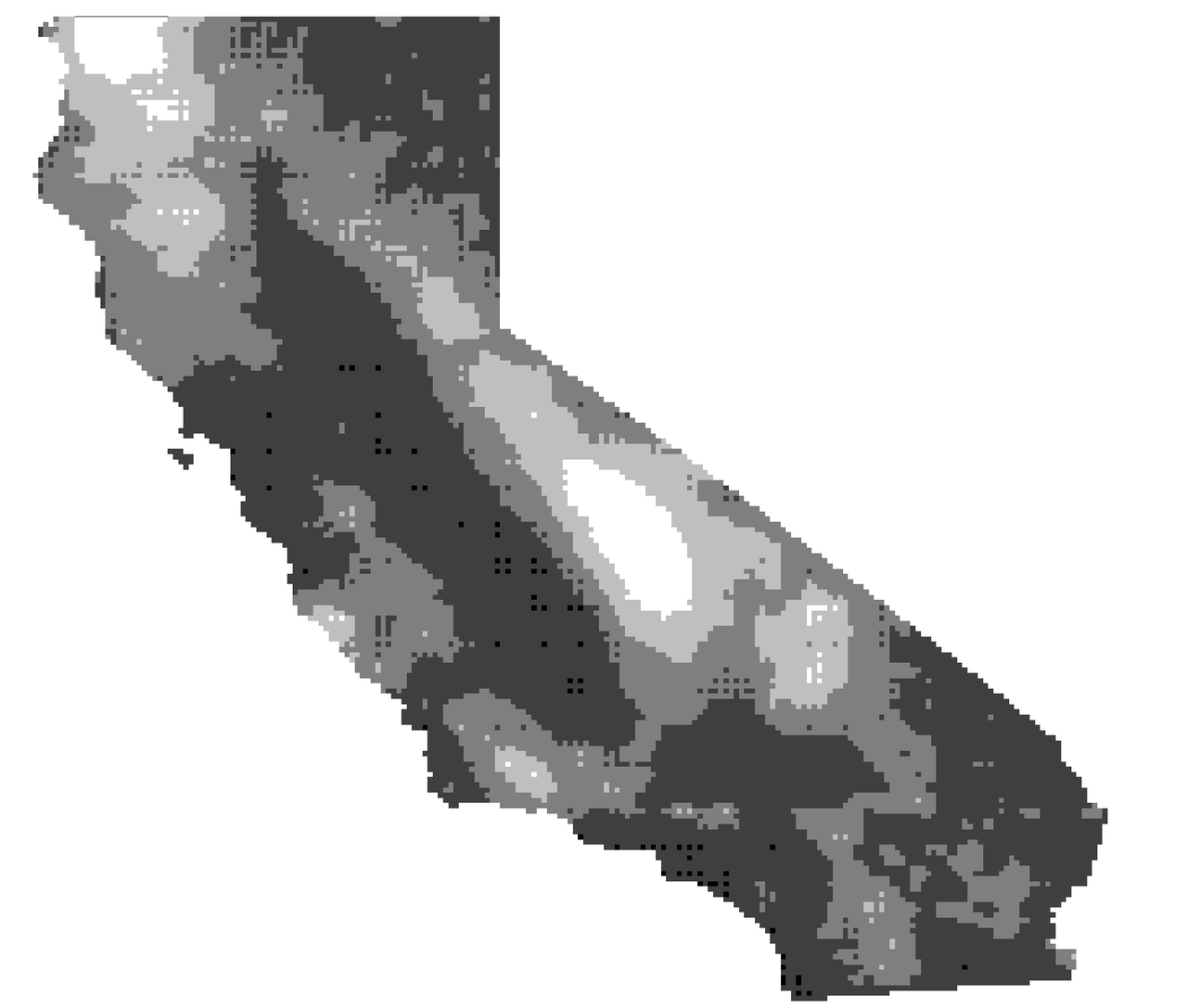
The order matters here and it is easy to get backwards. The zones were not drawn around terrain features and then measured. The surface was measured first, interpolated, and then cut where the data broke naturally. Terrain correspondence is a finding, and it is what makes the zones credible rather than convenient.
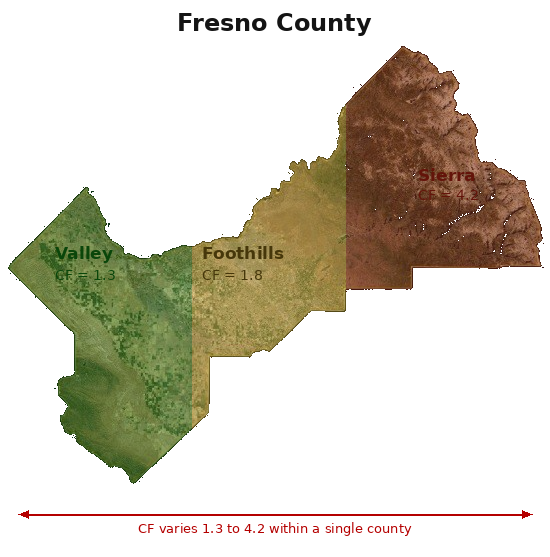
The obvious alternative partition is counties, because county boundaries are already in every dataset. They fail badly. Fresno County spans the flat Central Valley at 50 to 100 m, oak foothills at 300 to 800 m, and High Sierra above 4,000 m. Circuity inside that one county runs from 1.3 to 4.2. A county mean would be wrong for almost every location in it.
What the approximation buys and costs
Three methods compared against actual routed distances on all 435,848 routes.
| Method | MAE (km) | MAPE | Correlation |
|---|---|---|---|
| Uniform CF of 2.19 | 33.41 | 36.6% | 0.490 |
| Zone lookup | 26.81 | 29.2% | 0.690 |
| Origin-specific measurement | 25.74 | 28.2% | 0.716 |
Zones cut error by 20% relative to a uniform statewide assumption, and land within one percentage point of measuring every origin individually. That is the useful part: a five-value lookup table captures nearly everything a full per-origin measurement would, at a fraction of the storage and none of the query cost.
Held-out validation on 4,839 routes from 200 origins the model had never seen gives 31.8% MAPE overall, close enough to the in-sample 29.2% to trust the generalisation.
In deployment the zones are materialised into a lookup table of 1.53 million rows, joined to cluster centroids by nearest neighbour. At query time one indexed lookup returns the factor and it applies to every candidate distance at once. Thousands of routing calls become one join and a multiplication.
Where it breaks
Zone 5 is not reliable. On held-out data, zones 1 through 4 came within 6% of their defined values. Zone 5 was defined at 4.84 and measured at 3.62, with 100.5% MAPE. Remote mountain routing depends on which specific passes are open and on seasonal road conditions, and no static factor captures that. Zone 5 covers 231 of 4,839 held-out routes, so it is a small slice, and any answer that leans on it should be treated as indicative only.
Error grows monotonically with zone number. 15.2% in zone 1, 23.6%, 32.9%, 43.6%, then 100.5%. The method works best where it matters least, since flat accessible terrain was never the hard case. Zones 1 through 3 hold 81% of routes and stay under 33%.
29% MAPE is not small. Against a baseline of 119% error from using straight-line distance uncorrected, it is a large improvement. Against an actual routing call it is a real loss of precision, and whether that is acceptable depends entirely on the decision it feeds. For ranking candidate sites against each other, yes. For contracting a specific haul, no.
The factor is distance-independent, and it should not be. A single value per zone is applied to every haul from that zone regardless of length. That assumption turns out to be wrong in a specific and predictable way, which is the subject of the next post.
The road network is a snapshot. October 2024 OpenStreetMap. New roads, closures and seasonal restrictions are not reflected, and the zones do not know they are stale.
More on the transport method and how transport cost is reported.
References
Ballou, R.H., Rahardja, H. and Sakai, N. (2002). Selected Country Circuity Factors for Road Travel Distance Estimation. Transportation Research Part A, 36, 843–848.
Levinson, D. and El-Geneidy, A. (2009). The Minimum Circuity Frontier and the Journey to Work. Regional Science and Urban Economics.
Contreras, M. and Chung, W. (2016). Analysis of Transportation Costs in Forest Biomass Supply Chains.
Jenks, G.F. (1967). The Data Model Concept in Statistical Mapping. International Yearbook of Cartography, 7, 186–190.
OpenStreetMap contributors. Open Source Routing Machine.