Training an ML surrogate on a deterministic simulator
A deterministic simulator gives you unlimited labels with no measurement noise. That changes what R² means, how you sample, and what counts as validation.

Most models are trained on data someone measured. The labels are noisy, the measurement process has its own error, and a model that fits them too well is fitting the noise. Almost every instinct in supervised learning comes from that situation. When the labels come from a deterministic simulator instead, several of those instincts stop applying, and one of them becomes actively misleading.
The problem
The simulator being replaced computes forest harvest cost from terrain and biomass. It takes 1 to 4 milliseconds per evaluation, which is fast until you need 165 million of them to cover every cluster in California across every treatment and harvesting system. That is 23 to 92 hours of compute for one pass.
Runtime is the smaller issue. The larger one is that the downstream work needs the cost surface to exist as an object rather than a service. A Pareto sweep over cost and fire risk runs 13,860 optimisations. A conversational query has to answer in seconds. Neither can call a simulator, and neither wants to depend on the simulator's preprocessing stack being installed and configured.
So the goal is not a faster simulator. It is a portable artifact that behaves like the simulator and can be queried, joined, and shipped without it.
What a deterministic oracle changes
The simulator has no stochastic components. Same inputs, same outputs, every time. Three consequences follow, and they are worth separating because they pull in different directions.
Labels are free and unlimited. There is no annotation budget and no dataset to collect. You can generate as many examples as you can afford compute for, anywhere in the input space you want them. This is the pleasant part.
There is no noise to overfit. A model that fits the training labels exactly has not memorised measurement error, because there is no measurement error. It has approximated a function very well. The usual worry about a suspiciously high R² does not apply in the same way, though a different worry replaces it, discussed below.
Every error is attributable. A discrepancy between surrogate and simulator is pure approximation error. It is not variance to average away. In principle each one can be traced to a specific region of the input space where the model is underfitting, and validation does not need confidence intervals over repeated runs, because there is nothing to repeat.
That last point is the one worth carrying to other problems. The word for it is bias. Reporting a single RMSE over a test set treats the error as noise around a true value and quietly discards the information that matters: where the model is wrong, and by how much, in the regions people will actually query.
Sampling the input space
With a free oracle, the sampling design is a real decision rather than an accident of what data existed.
The obvious approach is to sample the input space uniformly. Enumerate plausible ranges for each of the 13 input features, sample a grid or a Latin hypercube, evaluate. This gives even coverage and it is wrong here, because it spends most of its budget on combinations that do not occur. Steep slope with high large-diameter biomass and short yarding distance is a valid point in feature space and not a real forest.
The approach taken instead samples the actual population: 500,000 georeferenced forest clusters from the state inventory, each evaluated across 11 treatments and every applicable harvesting system. That yields 40,923,870 labelled examples whose joint feature distribution matches the distribution the deployed model will see.
The tradeoff is explicit. Population sampling gives accuracy where it matters and leaves the model untested in feature-space regions that are physically possible but not currently observed. If California's forests change enough, the surrogate is extrapolating and nothing in its validation will warn you.
| Total | Share | |
|---|---|---|
| Examples generated | 40,923,870 | |
| Feasible | 15,343,319 | 37.5% |
| Infeasible | 25,580,551 | 62.5% |
That 62.5% is not a data quality problem. Those combinations have no cost because the operation cannot be performed: slope too steep for ground-based equipment, biomass too sparse to be worth moving, safety limits exceeded. Handling that split is its own design decision and its own post.
What the numbers mean
On 3,068,664 held-out feasible examples, the production model reaches R² = 0.9974, mean absolute error of $1.38 per green ton, and median absolute error of $0.73. Of predictions, 82.7% fall within $2 of the simulator's value, 95.8% within $5, and 98.7% within $10.
The R² deserves care. Against noisy labels, 0.9974 would be a red flag. Here it is a statement about function approximation quality and nothing else, and it is high because the underlying function is smooth and the feature set captures its inputs well. It says the surrogate reproduces the simulator. It says nothing about whether the simulator is right.
The dollar figures are more useful than the R², because they are in the units of the decision. A $1.38 mean error against costs averaging $65.68 per green ton is small relative to the differences between sites that a planner is choosing between.
One result cuts against the production choice and is worth stating plainly. A three-layer neural network scored better than the selected gradient boosting model on every accuracy metric: R² 0.9992 against 0.9974, mean absolute error $0.89 against $1.38, 98.9% within $5 against 95.8%. It was chosen against for latency, at 3.73 microseconds per prediction versus 0.73, which matters at 165 million predictions and in a query path.
There is a further wrinkle. The neural network was trained on a 2 million row subsample because of available memory, not because anyone decided that was enough data. Whether it would improve further on the full 15.3 million feasible examples is unknown. The comparison as run favours the production model's data advantage while the network still won on accuracy.
Validating the pipeline, not just the model
A held-out test set validates the model. It does not validate the inference pipeline, and those fail differently.
The model can be correct while the deployed system feeds it features computed slightly differently from the ones it trained on: a unit conversion applied twice, a join producing the wrong row, a default filling a null that was not null during training. Test-set metrics are blind to all of it, because the test set goes through the training pipeline.
The check for this: draw 100 combinations at random from the statewide inference output, run the actual simulator on those same combinations, compare. All 100 agreed within rounding. That confirms the features used at inference match the features used at training, which is a different claim from R² and a more fragile one.
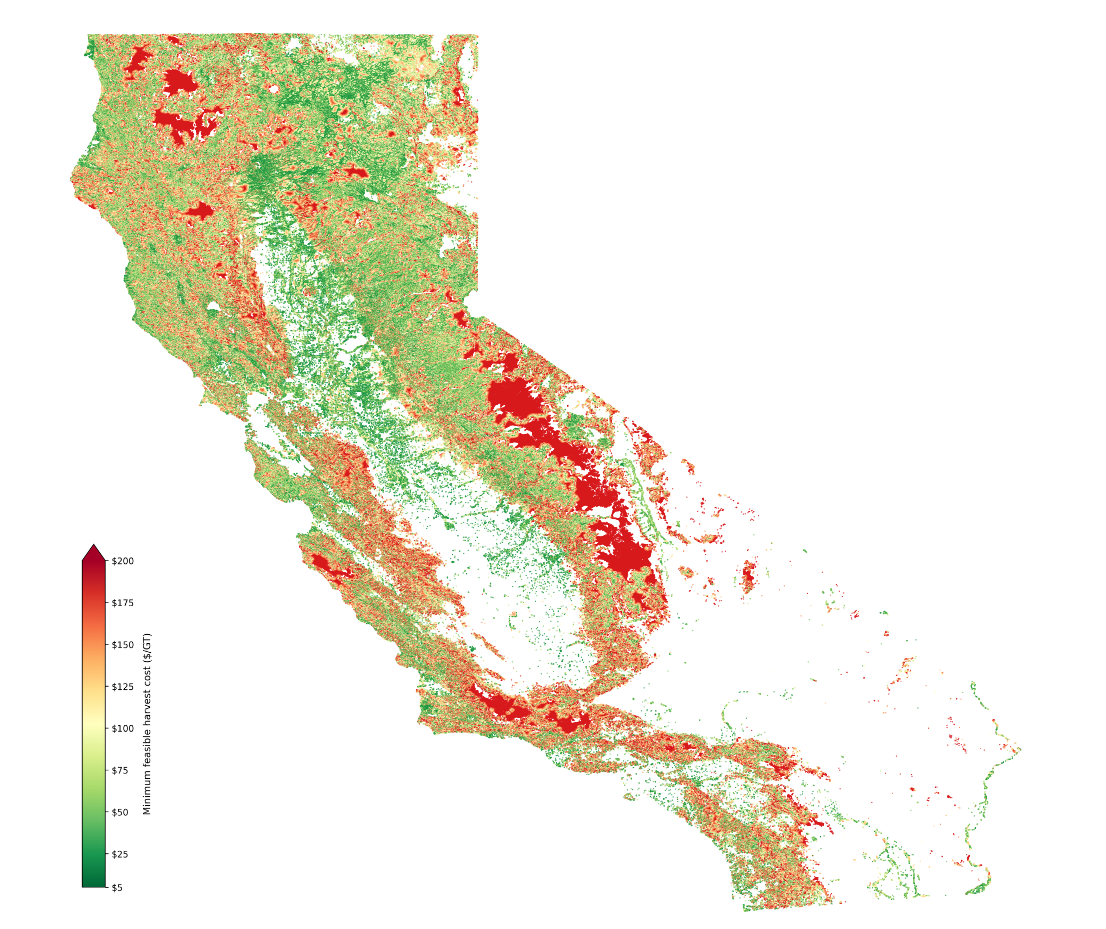
The full run scores 1.51 million clusters across 11 treatments and 10 harvesting systems in roughly 2 minutes on a workstation, and 1.16 million clusters have at least one feasible combination.
Where it breaks
The surrogate inherits every one of the simulator's assumptions. It is an approximation of a model, not of reality. If the simulator's production-rate equations are wrong for some stand type, the surrogate reproduces that error faithfully and with high confidence. Nothing in the validation can detect it, because the simulator is the ground truth by construction.
Accuracy is only demonstrated on the sampled population. Feature combinations outside the observed distribution are extrapolation. There is no out-of-distribution detection in the deployed layer.
The economic assumptions are frozen at training time. Fuel prices, wage rates and equipment cost indices were fixed when the labels were generated. That sounds like it would require retraining to change, and it does not, for a reason worth its own post.
A single error number hides the shape of the error. The threshold figures above are better than an RMSE and still aggregate across terrain, treatment and harvesting system. Which regimes carry the residual is a separate question.
Method details in the harvest cost documentation.
References
Fight, R.D., Hartsough, B.R. and Noordijk, P. (2006). Users Guide for FRCS: Fuel Reduction Cost Simulator Software. USDA Forest Service, Pacific Northwest Research Station.
Chen, T. and Guestrin, C. (2016). XGBoost: A Scalable Tree Boosting System. KDD '16, 785–794.
Queipo, N.V. et al. (2005). Surrogate-Based Analysis and Optimization. Progress in Aerospace Sciences, 41(1), 1–28.
Jenkins, J.C. et al. (2003). National-Scale Biomass Estimators for United States Tree Species. Forest Science, 49(1), 12–35.