Cheap fire risk reduction from a weighted objective
Weighting two objectives into one score is standard. The shape of the frontier is not: 5% weight toward fire buys 118.9% more risk reduction for 20.5% more cost.
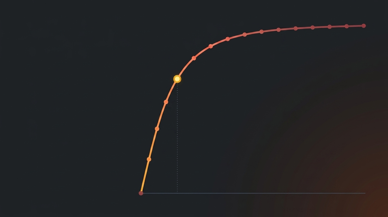
Combining two objectives that share no unit is a routine problem with a routine solution. Normalise both, pick a weight, sum them. The part that gets skipped is looking at the shape of the resulting frontier before choosing where to sit on it, and the shape here is lopsided enough to change the answer entirely. Five percent of the weight captures most of what the full weighting achieves.
The problem
A procurement optimiser selecting forest biomass by cost picks flat, accessible, nearby material. That is what cheap means. Those are also, systematically, not the places that burn.
The two objectives cannot be compared directly. One is dollars per tonne delivered. The other is annual burn probability multiplied by the biomass a treatment removes, which is a risk-reduction quantity with no natural price. There is no exchange rate between them, and inventing one is exactly the decision the weighting is trying to avoid making explicitly.
The standard move is scalarisation. Normalise both to a common range and combine them with a single parameter:
score_i = α * normalised_cost_i - (1 - α) * normalised_fire_efficiency_iAt α = 1 the optimiser minimises cost and ignores fire. At α = 0 it maximises fire risk reduction per dollar. Sort by score, select greedily until demand is met.
The weight is not a preference to be elicited. It is a knob whose response curve you have to measure before you can say anything useful about where to set it.
Sweeping the parameter
21 values of α, 60 candidate facility locations on a statewide grid, 11 treatments each. 13,860 optimisation runs, each building a full supply curve.
That sweep is only possible because the expensive parts were precomputed. Running the cost simulator and a routing engine inside each of 13,860 runs would put this analysis out of reach, which is the practical argument for surrogate layers: not that any single query gets faster, but that a class of analysis becomes affordable.
Define the leverage ratio as the percentage gain in fire risk reduction divided by the percentage cost premium, both relative to pure cost minimisation. It answers the question a decision maker actually has, which is what a dollar of extra spending buys.
| Fire weight | α | Cost ($/GT) | Cost premium | Fire gain | Leverage |
|---|---|---|---|---|---|
| 0% | 1.00 | 21.11 | — | — | — |
| 5% | 0.95 | 25.45 | +20.5% | +118.9% | 5.8× |
| 20% | 0.80 | 37.90 | +79.5% | +250.0% | 3.1× |
| 50% | 0.50 | 41.64 | +97.2% | +273.4% | 2.8× |
| 100% | 0.00 | 44.04 | +108.6% | +280.5% | 2.6× |
The first 5% of weight returns 5.8× leverage. By 20% weight the system has captured 89% of the maximum achievable fire gain, and leverage has already fallen to 3.1×. Going the rest of the way, from 20% weight to 100%, costs another 29 percentage points of premium to buy 30 percentage points of fire gain, at roughly break-even.
Why front-loading is the general case
This shape is not specific to fire and cost. Weighted-sum fronts over a large candidate pool are usually concave and usually front-loaded, and the mechanism is worth naming because it tells you where to look on your own problem.
The optimiser is choosing from a large set with heterogeneous performance on both objectives. Some candidates are good on both, some are good on one, most are mediocre. At zero weight on the second objective, the selection ignores a subpopulation that happens to score well on it at little cost penalty. Adding a small weight reorders the ranking just enough to pull those in. They are cheap because they were never far from being selected anyway.
Once that subpopulation is exhausted, further weight has to buy candidates that are genuinely expensive on the first objective. The slope collapses.
So the practical rule: the interesting operating point on a scalarised front is usually near the extreme, not near the middle. Sweeping at coarse intervals will miss it. Here a sweep at 0, 0.25, 0.5, 0.75, 1.0 would have shown a mild tradeoff and missed the entire finding, because everything interesting happens between α = 1.0 and α = 0.95.
Decomposing the premium
A 20.5% premium is a number without a lever attached. Splitting it by component gives one.
| Component | α = 1.0 | α = 0.95 | Change | Share of premium |
|---|---|---|---|---|
| Harvest | 15.21 | 15.38 | +0.17 | 8% |
| Transport | 5.89 | 7.94 | +2.05 | 92% |
| Total | 21.11 | 25.45 | +2.22 | 100% |
At the efficient point, 92% of the extra cost is hauling. Average road distance rises from 39.3 km to 53.0 km while harvest cost moves by 17 cents per tonne.
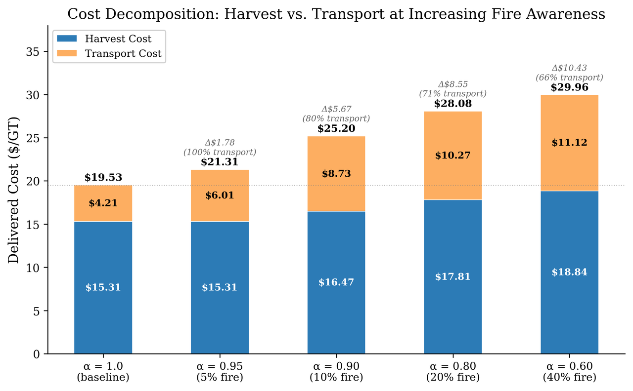
The interpretation is specific and it would not have been visible from the headline number. The optimiser is not switching to harder terrain. It is reaching further to find fire-prone clusters whose harvest economics are similar to what it was already buying. Fire-prone and expensive-to-harvest are less correlated than intuition suggests, and the binding constraint is road access.
That changes what a policy response looks like. An incentive of $3 to $5 per tonne for material sourced from high-risk areas is enough to trigger the shift, and it only has to compensate for hauling. No harvest-side subsidy is needed at the efficient point.
The ceiling
Under pure cost minimisation, 57% of selected clusters sit in the lowest burn probability tier. At 5% fire weighting that falls to 40%, and the combined High and Very High share rises from 18% to 33%.
Push the weighting all the way to α = 0 and the lowest tier climbs back to roughly 57%.
That non-monotonicity is the most important result in the chapter and the least comfortable one. With accurate road distances, the highest-risk terrain is remote enough that reaching it is prohibitively expensive, so the optimiser cannot redirect procurement as completely as the weighting suggests it should. Roughly half of procurement stays in low-risk areas no matter what the parameter says.
An earlier version of this analysis using straight-line distances did not show the ceiling. It appeared only once real road distances were used, which makes it a finding about the road network rather than about the optimiser.
Where this breaks
The scoring function is a choice, not a derivation. Min-max normalisation makes the weight sensitive to the range of each objective in the candidate pool, so α values are not comparable across regions with different cost distributions. A different normalisation gives a different curve and a different efficient point. The shape is robust. The specific value of 0.95 is not portable.
Untreatable clusters are excluded and they are the worst ones. Of 1.53 million clusters with valid burn probability, 371,000 have no feasible harvest system at all, and their mean burn probability is 17% higher than treatable clusters. The places most in need of fuel reduction are disproportionately the places conventional harvesting cannot reach. Every number above is conditional on that exclusion.
Burn probability is a static snapshot. 2020 to 2022 landscape conditions. The analysis does not model how treating a cluster changes fire behaviour on the surrounding landscape, which is the actual mechanism by which fuel treatment reduces risk. Fire risk reduction here is a proxy quantity, not a simulated outcome.
Each year is independent. No temporal compounding, no accounting for a treated cluster's reduced risk in later years.
The fire risk reduction metric is proportional to biomass removed. That embeds an assumption that removing twice the material halves risk twice as much, which is not how fuel loading works.
More on the fire method and how the tradeoff is presented.
References
Scott, J.H. et al. (2024). Wildfire Risk to Communities. USDA Forest Service.
Finney, M.A. et al. (2011). A Method for Ensemble Wildland Fire Simulation. Environmental Modeling and Assessment, 16, 153–167.
California Legislative Analyst's Office (2018). Improving California's Forest and Watershed Management.
California Public Utilities Commission. BioRAM and BioMAT program documentation.